Tangent field

import importlib
import time

import matplotlib.pyplot as plt

import nannos as nn
from nannos.formulations.tangent import get_tangent_field

bk = nn.backend
plt.close("all")
# plt.ion()

We will generate a field tangent to the material interface

scale = 1.5
nh = 600
lattice = nn.Lattice(([1 * scale, 0], [0, scale]), discretization=2**9)

x, y = lattice.grid
circ = lattice.ellipse(
    (0.3 * scale, 0.3 * scale), (0.1 * scale, 0.25 * scale), rotate=-30
)
rect = lattice.rectangle(
    (0.7 * scale, 0.7 * scale), (0.2 * scale, 0.5 * scale), rotate=20
)
grid = lattice.ones() * (3 + 0.01j)
grid[circ] = 1
grid[rect] = 1

st = lattice.Layer("pat", thickness=scale, epsilon=grid)
lays = [lattice.Layer("sup"), st, lattice.Layer("sub")]
pw = nn.PlaneWave(wavelength=1 / 1.2)
sim = nn.Simulation(lays, pw, nh)

FFT version

rfilt = 2
dsp = 10
t0 = -time.time()
t = get_tangent_field(
    lattice, grid, sim.harmonics, normalize=False, type="fft", rfilt=rfilt
)
t0 += time.time()
print(f"Elapsed time {t0:.4f}s")


plt.figure()
st.plot()
plt.quiver(
    x[::dsp, ::dsp],
    y[::dsp, ::dsp],
    t[0][::dsp, ::dsp],
    t[1][::dsp, ::dsp],
    scale=11,
)
plt.axis("scaled")
_ = plt.axis("off")
plt.show()

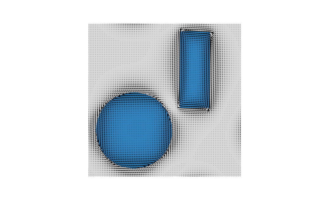
Elapsed time 0.0634s

FFT version (normalized)

t0 = -time.time()
tnorma = get_tangent_field(
    lattice, grid, sim.harmonics, normalize=True, type="fft", rfilt=rfilt
)
t0 += time.time()
print(f"Elapsed time {t0:.4f}s")


plt.figure()
st.plot()
plt.quiver(
    x[::dsp, ::dsp],
    y[::dsp, ::dsp],
    tnorma[0][::dsp, ::dsp],
    tnorma[1][::dsp, ::dsp],
    scale=50,
)
plt.axis("scaled")
_ = plt.axis("off")
plt.show()

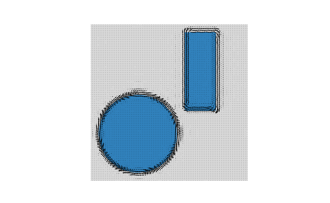
Elapsed time 0.0601s

Estimated memory usage: 727 MB