Tutorials#

Basic Example#

This basic example demonstrates key features of nannos.

First import the package.

import nannos as nn

Create the lattice.

lattice = nn.Lattice(basis_vectors = [[1.0, 0], [0, 1.0]], discretization=2**9)

Define the layers. The thickness for the semi infinite input and output media is irrelevant.

sup = lattice.Layer("Superstrate", epsilon=1)
ms = lattice.Layer("Metasurface", thickness=0.5)
sub = lattice.Layer("Substrate", epsilon=2)

Create the permittivity pattern for the structured layer.

ms.epsilon = lattice.ones() * 12.0
circ = lattice.circle(center=(0.5, 0.5), radius=0.2)
ms.epsilon[circ] = 1

Define the layer stack as a list from input medium to output medium.

stack = [sup, ms, sub]

Define the incident plane wave.

pw = nn.PlaneWave(wavelength=0.9, angles=(0, 0, 0))

Create the simulation.

sim = nn.Simulation(stack, pw, nh=200)

Plot the unit cell.

p = sim.plot_structure()
p.show_axes()
p.show(jupyter_backend='panel')

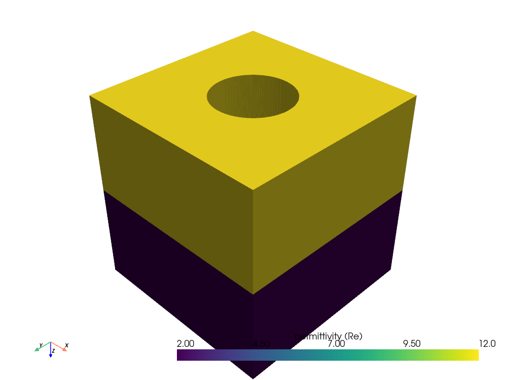
Compute the reflection and transmission:

R,T = sim.diffraction_efficiencies()
print("reflection: ", R)
print("transmission: ", T)
print("sum :", R + T)

reflection:  0.3271754877303915
transmission:  0.6728245122696163
sum : 1.0000000000000078