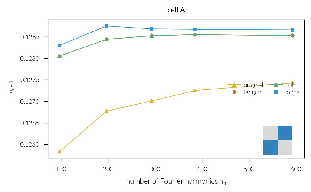
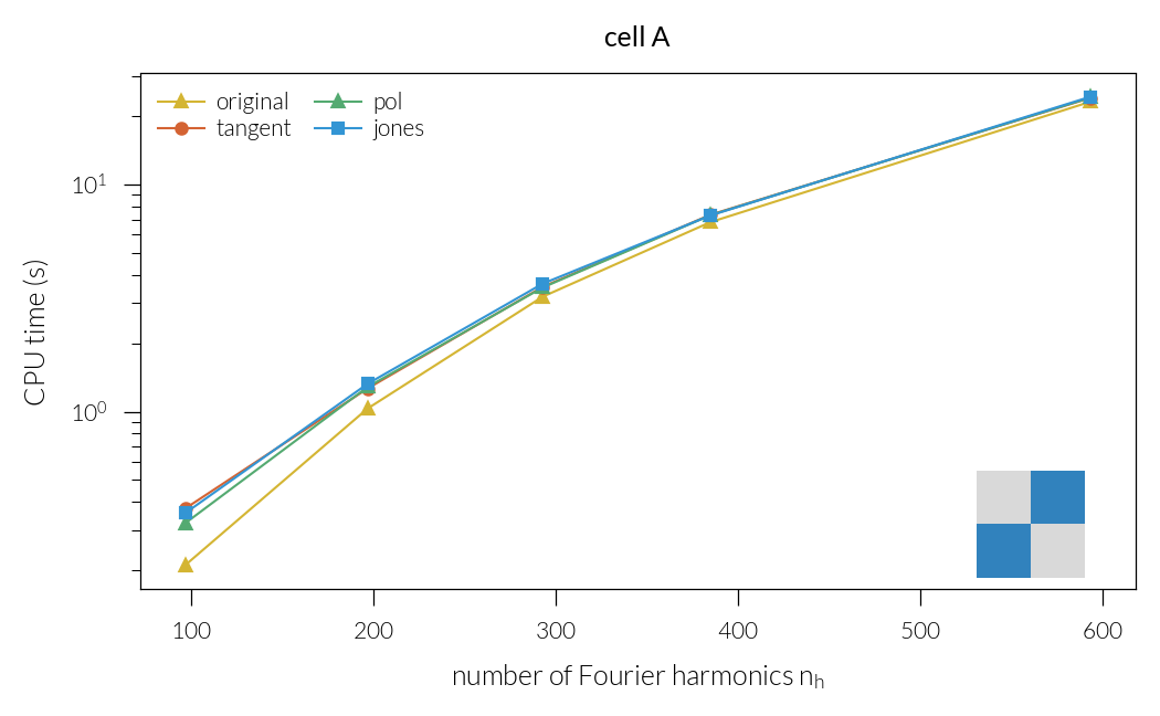
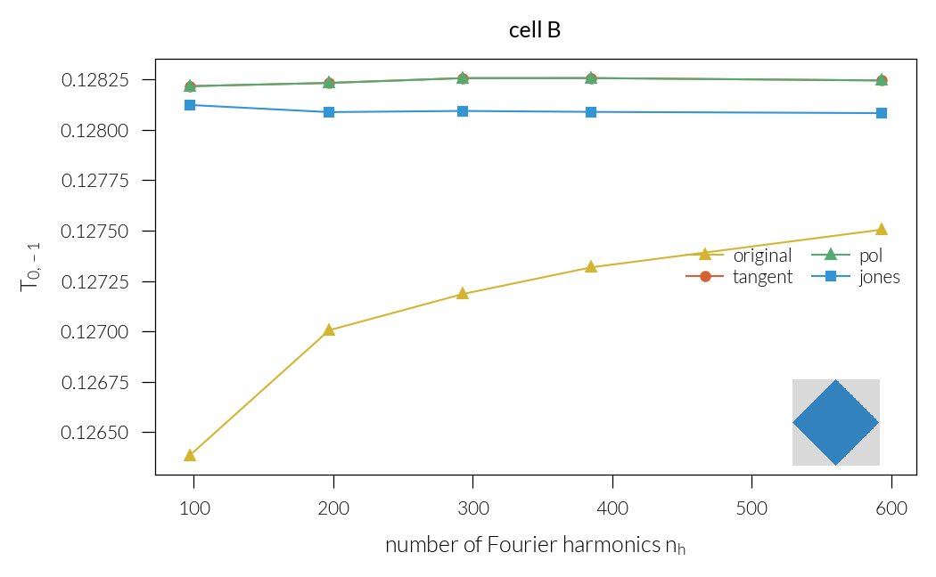
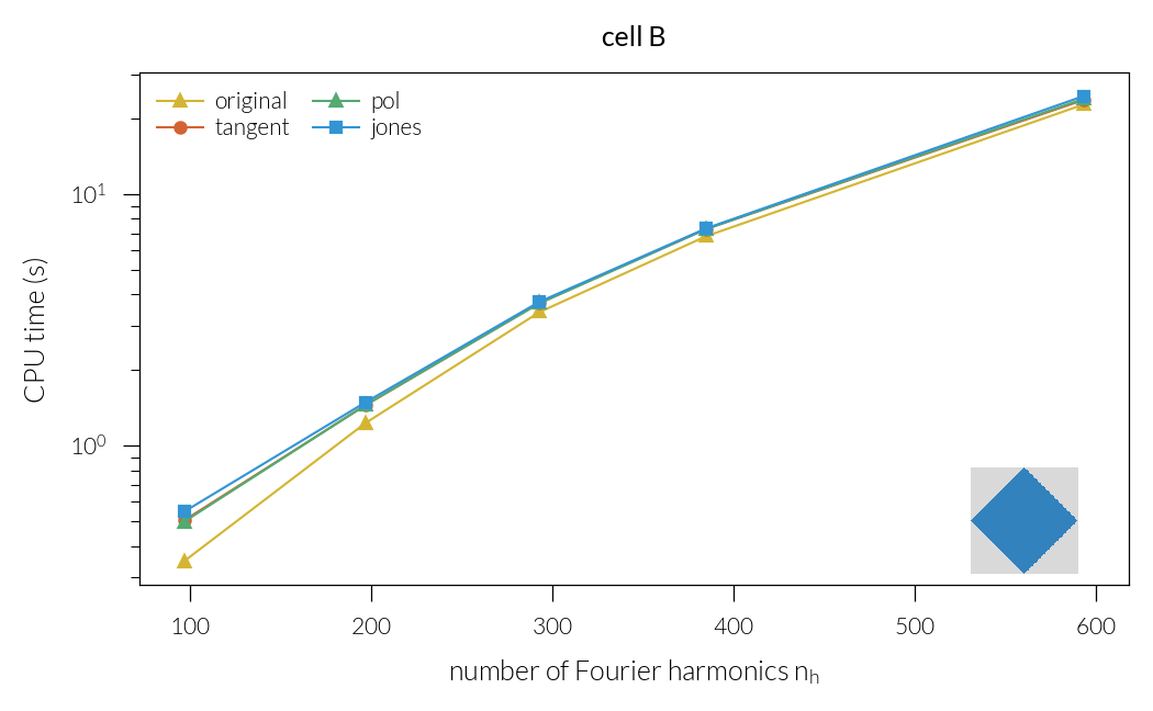
Convergence

Convergence of the various FMM formulations.

import matplotlib.pyplot as plt
import numpy as np

import nannos as nn

We will study the convergence on a benchmark case from [Li1997]. First we define the main function that performs the simulation.

def checkerboard(nh, formulation):
    la = 1
    d = 2 * 1.25 * la
    Nx = 2**9
    Ny = 2**9
    lattice = nn.Lattice(([d, 0], [0, d]), discretization=(Nx, Ny))
    pw = nn.PlaneWave(wavelength=la, angles=(0, 0, 0))
    epsgrid = lattice.ones() * 2.25
    sq1 = lattice.square((0.25 * d, 0.25 * d), 0.5 * d)
    sq2 = lattice.square((0.75 * d, 0.75 * d), 0.5 * d)
    epsgrid[sq1] = 1
    epsgrid[sq2] = 1

    sup = lattice.Layer("Superstrate", epsilon=2.25)
    sub = lattice.Layer("Substrate", epsilon=1)
    st = lattice.Layer("Structured", la)
    st.epsilon = epsgrid

    sim = nn.Simulation([sup, st, sub], pw, nh, formulation=formulation)
    order = (
        -1,
        -1,
    )  # this actually corresponds to order (0,-1) for the other unit cell in [Li1997]
    R, T = sim.diffraction_efficiencies(orders=True)
    t = sim.get_order(T, order)
    return R, T, t, sim

Perform the simulation for different formulations and number of retained harmonics:

NH = [100, 200, 300, 400, 600]
formulations = ["original", "tangent", "pol", "jones"]
nhs = {f: [] for f in formulations}
ts = {f: [] for f in formulations}


for nh in NH:
    print("============================")
    print("number of harmonics = ", nh)
    print("============================")

    for formulation in formulations:
        Ri, Ti, t, sim = checkerboard(nh, formulation=formulation)
        R = np.sum(Ri)
        T = np.sum(Ti)
        print("formulation = ", formulation)
        print("nh0 = ", nh)
        print("nh = ", sim.nh)
        print("t = ", t)
        print("R = ", R)
        print("T = ", T)
        print("R+T = ", R + T)
        print("-----------------")
        nhs[formulation].append(sim.nh)
        ts[formulation].append(t)

Out:

============================
number of harmonics =  100
============================
formulation =  original
nh0 =  100
nh =  97
t =  0.125834435458293
R =  0.10288332489073707
T =  0.8971166751093032
R+T =  1.0000000000000402
-----------------
formulation =  tangent
nh0 =  100
nh =  97
t =  0.12789483284988978
R =  0.10772217772672452
T =  0.8932679641845813
R+T =  1.0009901419113059
-----------------
formulation =  pol
nh0 =  100
nh =  97
t =  0.1278948328498899
R =  0.10772217772672323
T =  0.8932679641845804
R+T =  1.0009901419113036
-----------------
formulation =  jones
nh0 =  100
nh =  97
t =  0.12778179271105744
R =  0.10636770408199606
T =  0.8938165896212739
R+T =  1.0001842937032699
-----------------
============================
number of harmonics =  200
============================
formulation =  original
nh0 =  200
nh =  197
t =  0.1267736966566054
R =  0.10235840915154018
T =  0.8976415908484603
R+T =  1.0000000000000004
-----------------
formulation =  tangent
nh0 =  200
nh =  197
t =  0.12847737576679555
R =  0.1054678332527112
T =  0.8946672545568912
R+T =  1.0001350878096025
-----------------
formulation =  pol
nh0 =  200
nh =  197
t =  0.12847737576679297
R =  0.10546783325265274
T =  0.8946672545568815
R+T =  1.000135087809534
-----------------
formulation =  jones
nh0 =  200
nh =  197
t =  0.1281760637084313
R =  0.10509028793764244
T =  0.8949291721191834
R+T =  1.000019460056826
-----------------
============================
number of harmonics =  300
============================
formulation =  original
nh0 =  300
nh =  293
t =  0.1270087978399685
R =  0.10188104131998693
T =  0.8981189586800109
R+T =  0.9999999999999978
-----------------
formulation =  tangent
nh0 =  300
nh =  293
t =  0.1285086549442586
R =  0.10449511205454168
T =  0.8951914153031378
R+T =  0.9996865273576795
-----------------
formulation =  pol
nh0 =  300
nh =  293
t =  0.12850865494425495
R =  0.1044951120544991
T =  0.8951914153031264
R+T =  0.9996865273576255
-----------------
formulation =  jones
nh0 =  300
nh =  293
t =  0.1283292326074173
R =  0.1042030169610986
T =  0.8959004035788981
R+T =  1.0001034205399968
-----------------
============================
number of harmonics =  400
============================
formulation =  original
nh0 =  400
nh =  385
t =  0.1272505400763357
R =  0.10155950454446896
T =  0.8984404954555192
R+T =  0.9999999999999881
-----------------
formulation =  tangent
nh0 =  400
nh =  385
t =  0.1285429912819176
R =  0.1038136984253561
T =  0.8963555928354342
R+T =  1.0001692912607902
-----------------
formulation =  pol
nh0 =  400
nh =  385
t =  0.12854299128190805
R =  0.10381369842564905
T =  0.8963555928354161
R+T =  1.0001692912610651
-----------------
formulation =  jones
nh0 =  400
nh =  385
t =  0.12842243009077275
R =  0.10367976392139656
T =  0.8963775054546795
R+T =  1.000057269376076
-----------------
============================
number of harmonics =  600
============================
formulation =  original
nh0 =  600
nh =  593
t =  0.1274294323989556
R =  0.10144409729530053
T =  0.8985559027045601
R+T =  0.9999999999998607
-----------------
formulation =  tangent
nh0 =  600
nh =  593
t =  0.12853414900493945
R =  0.10332104034623943
T =  0.8965903301716726
R+T =  0.999911370517912
-----------------
formulation =  pol
nh0 =  600
nh =  593
t =  0.1285341490049613
R =  0.10332104034624846
T =  0.8965903301716955
R+T =  0.999911370517944
-----------------
formulation =  jones
nh0 =  600
nh =  593
t =  0.1284325735090812
R =  0.1032580794147723
T =  0.8967923934378219
R+T =  1.0000504728525943
-----------------

Plot the results:

markers = {"original": "^", "tangent": "o", "jones": "s", "pol": "^"}
colors = {
    "original": "#d4b533",
    "tangent": "#d46333",
    "jones": "#3395d4",
    "pol": "#54aa71",
}

for formulation in formulations:
    plt.plot(
        nhs[formulation],
        ts[formulation],
        "-",
        color=colors[formulation],
        marker=markers[formulation],
        label=formulation,
    )
    plt.pause(0.1)
plt.legend()
plt.xlabel("number of Fourier harmonics $n_h$")
plt.ylabel("$T_{0,-1}$")
plt.ylim(0.1255, 0.129)
plt.tight_layout()

Out:

/builds/nannos/nannos.gitlab.io/nannos/examples/basic/plot_convergence.py:106: UserWarning: FigureCanvasAgg is non-interactive, and thus cannot be shown
  plt.pause(0.1)

Estimated memory usage: 2649 MB