One dimensional grating

Convergence.

import matplotlib.pyplot as plt
import numpy as np

import nannos as nn

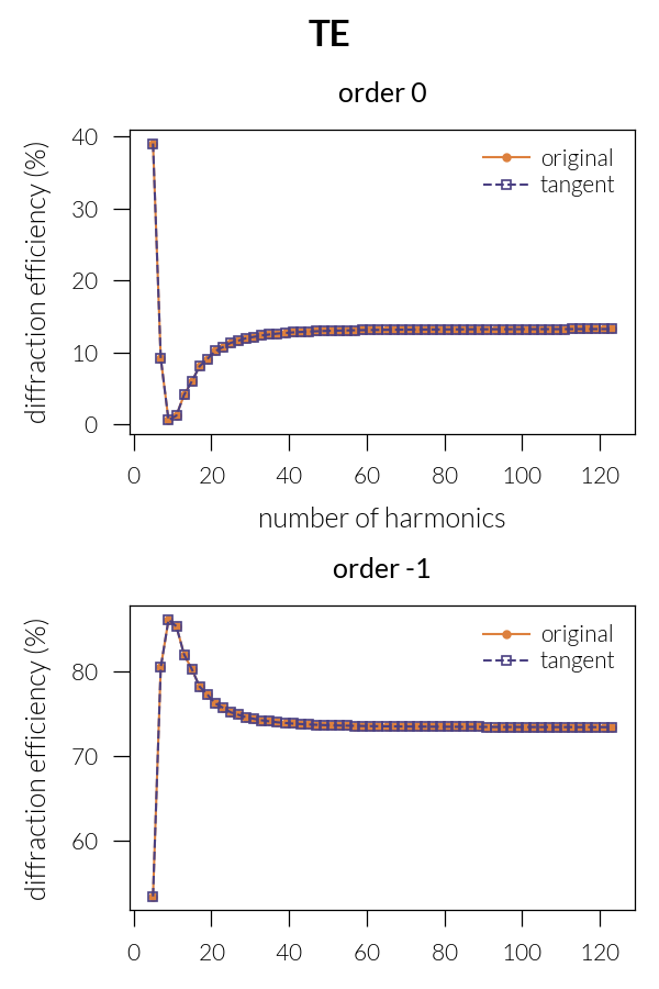
We will study the 1D metallic grating as in [Li1993].

def convergence_study(form, psi, Nh):
    ts0 = []
    tsm1 = []
    ns = []
    for nh in Nh:
        lattice = nn.Lattice(1, 2**9)
        eps_metal = (0.22 + 6.71j) ** 2
        epsgrid = lattice.ones() * 1
        hole = lattice.stripe(0.5, 0.5)
        epsgrid[hole] = eps_metal
        sup = lattice.Layer("Superstrate")
        sub = lattice.Layer("Substrate", epsilon=eps_metal)
        grating = lattice.Layer("Grating", thickness=1)
        grating.epsilon = epsgrid
        stack = [sup, grating, sub]
        pw = nn.PlaneWave(wavelength=1, angles=(30, 0, psi))
        sim = nn.Simulation(stack, pw, nh, formulation=form)
        R, T = sim.diffraction_efficiencies()
        Ri, Ti = sim.diffraction_efficiencies(orders=True)
        R0 = sim.get_order(Ri, 0)
        Rm1 = sim.get_order(Ri, -1)
        ts0.append(R0)
        tsm1.append(Rm1)
        ns.append(sim.nh)
    return np.array(ns), 100 * np.array(ts0), 100 * np.array(tsm1)


def run(psi):
    Nh = range(5, 125, 2)
    fig, ax = plt.subplots(2, 1, figsize=(2.0, 3.0))
    title = "TM" if psi == 0 else "TE"
    ns, ts0, tsm1 = convergence_study("original", psi, Nh)
    ax[0].plot(ns, ts0, "-o", label="original", c="#dd803d", ms=1)
    ax[1].plot(ns, tsm1, "-o", label="original", c="#dd803d", ms=1)
    ns_tan, ts0_tan, tsm1_tan = convergence_study("tangent", psi, Nh)
    ax[0].plot(
        ns_tan, ts0_tan, "--s", label="tangent", c="#4a4082", ms=2, mew=0.4, mfc="None"
    )
    ax[1].plot(
        ns_tan, tsm1_tan, "--s", label="tangent", c="#4a4082", ms=2, mew=0.4, mfc="None"
    )
    ax[0].set_title("order 0")
    ax[1].set_title("order -1")
    ax[0].legend()
    ax[1].legend()
    ax[0].set_xlabel("number of harmonics")
    ax[0].set_ylabel("diffraction efficiency (%)")
    ax[1].set_ylabel("diffraction efficiency (%)")
    plt.suptitle(title, weight="bold", size=8)
    plt.tight_layout()
    plt.pause(0.1)

For TE polarization the two formulations are equivalent:

run(psi=90)

Out:

/builds/nannos/nannos.gitlab.io/nannos/examples/basic/plot_1d_grating.py:77: UserWarning: FigureCanvasAgg is non-interactive, and thus cannot be shown
  plt.pause(0.1)

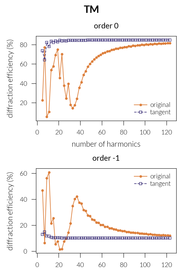
We can see that in TM polarization, the convergence is greatly improved by using proper Fourier factorization rules implemented by the tangent formulation.

run(psi=0)

Out:

/builds/nannos/nannos.gitlab.io/nannos/examples/basic/plot_1d_grating.py:77: UserWarning: FigureCanvasAgg is non-interactive, and thus cannot be shown
  plt.pause(0.1)

Estimated memory usage: 131 MB