Permittivity approximation

Get the Fourier representation of the permittivity as a function of number of harmonics.

import matplotlib.pyplot as plt
import numpy as np

import nannos as nn

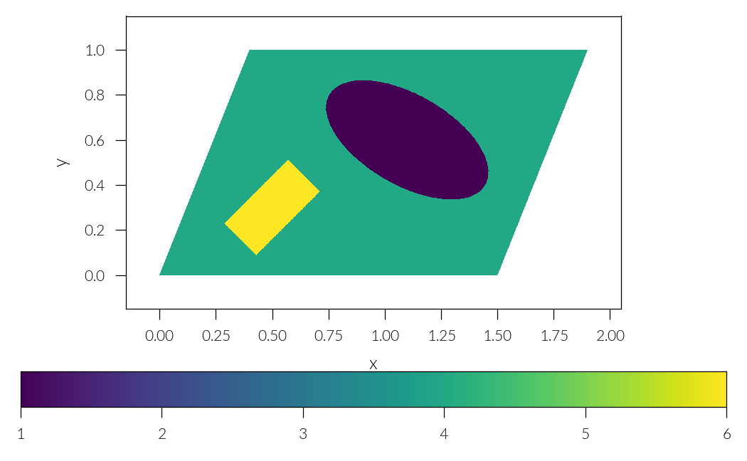
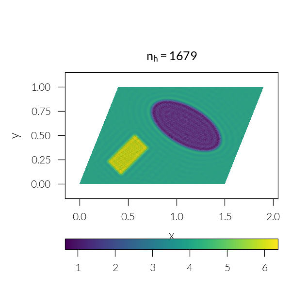
lattice = nn.Lattice([[1.5, 0], [0.4, 1]], discretization=(2**10, 2**10))
sup = lattice.Layer("Superstrate", epsilon=1)
sub = lattice.Layer("Substrate", epsilon=1)
hole = lattice.ellipse(center=(1.1, 0.6), radii=(0.2, 0.4), rotate=60)
incl = lattice.rectangle(center=(0.5, 0.3), widths=(0.2, 0.4), rotate=-45)
epsilon = lattice.ones() * 4
epsilon[hole] = 1
epsilon[incl] = 6
ms = lattice.Layer("Metasurface", thickness=0.5, epsilon=epsilon)
pw = nn.PlaneWave(wavelength=1.5, angles=(0, 0, 0))

Lets first plot the permmitivity we want to approximate

plt.figure()
ims = ms.plot(cmap="viridis")
plt.xlabel("$x$")
plt.ylabel("$y$")
plt.colorbar(ims[0], orientation="horizontal")
plt.tight_layout()

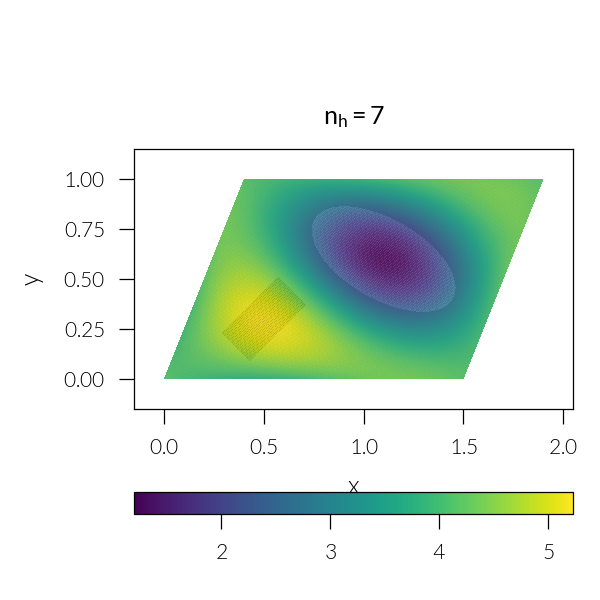
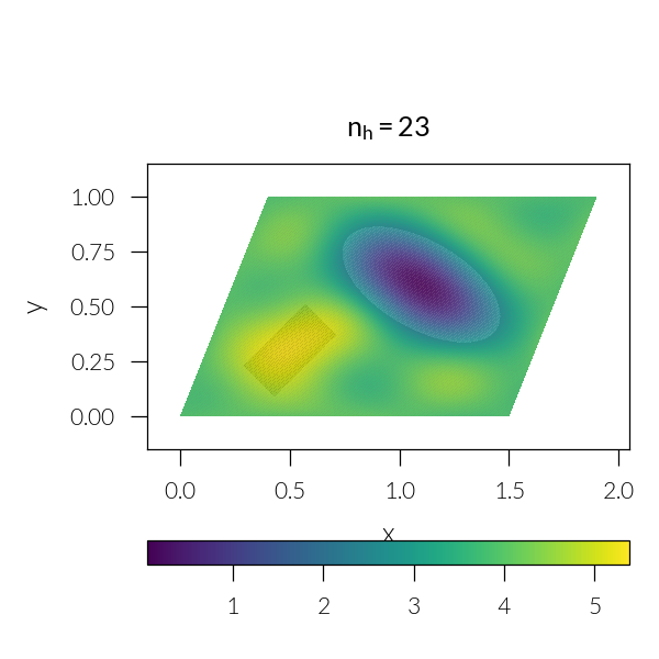
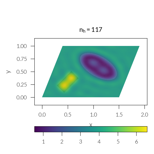
Loop through number of harmonics

for n in [3, 5, 7, 11, 21, 41]:
    sim = nn.Simulation([sup, ms, sub], pw, nh=n**2)
    eps = sim.get_epsilon(ms)
    plt.figure(figsize=(2, 2))
    approx = plt.pcolormesh(*lattice.grid, eps.real)
    ims = ms.plot(alpha=0.1, cmap="Greys")
    plt.xlabel("$x$")
    plt.ylabel("$y$")
    plt.colorbar(approx, orientation="horizontal")
    plt.title(rf"$n_h = {sim.nh}$")
    plt.tight_layout()

• 
• 
• 
• 
• 
• 

Estimated memory usage: 187 MB